Tutorial 5 - NMR Properties: using Soprano for working with .magres files#
      _
    /|_|\
   / / \ \
  /_/   \_\
  \ \   / /
   \ \_/ /
    \|_|/
SOPRANO: a Python library for generation, manipulation and analysis of large batches of crystalline structures
Developed within the CCP-NC project. Copyright STFC 2022
# Basic imports
import os, sys
sys.path.insert(0, os.path.abspath('..')) # This to add the Soprano path to the PYTHONPATH
                                          # so we can load it without installing it
# Other useful imports

import numpy as np

import ase
from ase import io as ase_io

%matplotlib inline
import matplotlib.pyplot as plt
plt.ion()

%reload_ext autoreload
%autoreload 2
1 - Loading magres files#
ASE can read the Magres file format from version 3.11.0 (~2016). If your version of ASE does not support loading Magres files, try updating it or download the bleeding edge version from GitLab:
C2H6O = ase_io.read('tutorial_data/ethanol.magres')
2 - Labels and indices#
Labels and indices used in the magres file are stored in their own arrays and can be easily accessed and used to select atoms.
If you use CASTEP and obtain your initial structure from a CIF file, note that you can use cif2cell with the --export-cif-labels flag to use the CIF site labels in your CASTEP .cell file. These labels will then be output in the generated .magres file.
labels = C2H6O.get_array('labels')
indices = C2H6O.get_array('indices')

# Select only the protons' indices
H_i = np.where(labels == 'H')[0]
H = C2H6O[H_i]
# Select only C2
C2_i = np.where((labels == 'C') & (indices == 2))[0]
C2 = C2H6O[C2_i]

print("There are {0} hydrogen atom(s)".format(len(H)))
print("The C2 atom is positioned at x = {0}, y = {1}, z = {2} Ang".format(*C2.get_positions()[0]))
There are 6 hydrogen atom(s)
The C2 atom is positioned at x = -0.247915, y = 1.164107, z = 0.937396 Ang
# Soprano provides a way to generate Jmol/MagresView-style labels from the atoms object:
from soprano.properties.labeling import MagresViewLabels
jmol_labels = MagresViewLabels.get(C2H6O)

# One can also recreate the Jmol/MagresView-style labels manuall if needed:
# jmol_labels = ["{0}_{1}".format(l, i) for l, i in zip(labels, indices)]

print("The labels are {0}".format(', '.join(jmol_labels)))
The labels are H_1, H_2, H_3, H_4, H_5, H_6, C_1, C_2, O_1
If you had labels in your CASTEP .cell file (e.g. via cif2cell from a CIF file), then your magres file should already have labels in them. In that case, they get loaded as an array automatically by the ASE parser.
For example, the EDIZUM.magres file has CIF-style labels with four copies of each label corresponding to the four molecules in the unit cell.
edizum = ase_io.read("tutorial_data/EDIZUM.magres")
# You can access the labels array like this:
edizum_labels = edizum.get_array("labels")

print(f"There are {len(edizum_labels)} labels - one for each site.")
print(f"but there are only {len(np.unique(edizum_labels))} unique labels since there are four molecules per cell.")
print(f"\nThe unique labels are: \n{np.unique(edizum_labels)}")
There are 148 labels - one for each site.
but there are only 37 unique labels since there are four molecules per cell.

The unique labels are:
['C1' 'C10' 'C11' 'C12' 'C13' 'C14' 'C15' 'C2' 'C3' 'C4' 'C5' 'C6' 'C7'
 'C8' 'C9' 'H1' 'H10' 'H11' 'H12' 'H13' 'H14' 'H15' 'H16' 'H17' 'H18'
 'H19' 'H2' 'H3' 'H4' 'H5' 'H6' 'H7' 'H8' 'H9' 'N1' 'O1' 'O2']
3 - Magnetic shieldings and chemical shifts#
All the NMR tensors stored in the original .magres file are saved as arrays in the Atoms object and can be accessed directly. However, Soprano also provides a set of properties to express the tensors in the form of parameters useful to compute the spectrum.
from soprano.properties.nmr import *

# Isotropy, Anisotropy and Asymmetry (Haeberlen convention)
# These return arrays of the same length as the number of atoms.
iso = MSIsotropy.get(C2H6O)
aniso = MSAnisotropy.get(C2H6O)
asymm = MSAsymmetry.get(C2H6O)

print('Label\tIsotropy\tAnisotropy\tAsymmetry')
for i, jl in enumerate(jmol_labels):
    print('{0}\t{1:6.2f} ppm\t{2:6.2f} ppm\t{3:3.2f}'.format(jl, iso[i], aniso[i], asymm[i]))
Label	Isotropy	Anisotropy	Asymmetry
H_1	 29.59 ppm	  8.94 ppm	0.14
H_2	 30.26 ppm	  8.19 ppm	0.21
H_3	 30.10 ppm	  7.29 ppm	0.06
H_4	 26.98 ppm	  8.17 ppm	0.94
H_5	 27.39 ppm	 -7.12 ppm	0.93
H_6	 31.98 ppm	 14.12 ppm	0.45
C_1	156.47 ppm	 33.80 ppm	0.70
C_2	109.86 ppm	 70.25 ppm	0.41
O_1	268.03 ppm	-51.38 ppm	0.98
# Span and skew
span = MSSpan.get(C2H6O)
skew = MSSkew.get(C2H6O)

print('Label\t  Span\t\t Skew')
for i, jl in enumerate(jmol_labels):
    print('{0}\t{1:6.2f} ppm\t{2:6.2f}'.format(jl, span[i], skew[i]))
Label	  Span		 Skew
H_1	  9.36 ppm	  0.82
H_2	  8.76 ppm	  0.74
H_3	  7.43 ppm	  0.92
H_4	 10.72 ppm	  0.05
H_5	  9.33 ppm	 -0.05
H_6	 16.25 ppm	  0.48
C_1	 41.73 ppm	  0.24
C_2	 79.95 ppm	  0.51
O_1	 68.22 ppm	 -0.01
Magnetic shielding Euler angles are discussed in more detail below, but as a quick example, you can extract the MS Euler angles like this:
from soprano.properties.nmr import MSEuler
# This defaults to Haeberlen convention, ZYZ, active rotation. To learn more about these conventions, see the Euler angle section below.
all_eulers=  MSEuler.get(C2H6O)
print("MS Euler angles in degrees:")
print(all_eulers * 180 / np.pi)
MS Euler angles in degrees:
[[ 27.96235601  45.33901509  26.83660999]
 [272.66415652  77.36879495  93.22520173]
 [182.04368043  35.14497966 166.45558554]
 [182.66142427  83.1949885  115.14989736]
 [191.97626819  50.93125971 125.47393484]
 [299.07186816  42.28810672  25.35033859]
 [ 93.10412193  47.43018725 152.96615397]
 [  9.25627104  54.93258925  41.36551806]
 [183.04713505  59.54692522 125.9519578 ]]
MS shielding conventions#
There are many different conventions used to describe the magnetic shielding tensors. These are nicely explained here: http://anorganik.uni-tuebingen.de/klaus/nmr/index.php?p=conventions/csa/csa
and in the Soprano documentation.
There are some convenience methods in Soprano to get descriptions of the MS tensor according to different conventions. First we can extract a list of MagneticShielding objects from the Atoms object, then we can use different methods to get the tensor in different conventions.
mstensors = MSTensor.get(C2H6O)
ms0 = mstensors[0]
print(ms0.iupac_values, '\n')
# print(ms0.mehring_values, '\n')
print(ms0.haeberlen_values, '\n')
print(ms0.herzfeldberger_values, '\n')
IUPACNotaion/MehringNotation:
  sigma_11:  26.18898
  sigma_22:  27.03525
  sigma_33:  35.55363
  sigma_iso: 29.59262

HaeberlenNotation:
  sigma_iso (isotropy): 29.59262
  sigma (reduced anisotropy): 5.96101
  delta (anisotropy): 8.94151
  eta (asymmetry): 0.14197

HerzfeldBergerNotation/MarylandNotation:
  sigma_iso (isotropy): 29.59262
  omega (span):     9.36465
  kappa (skew):     0.81926
print(ms0)
Magnetic Shielding Tensor for H:
[[30.29818, 1.20511, 3.67274],
 [ 1.96313,27.57653, 2.57545],
 [ 4.21834, 2.16271,30.90315]]
HaeberlenNotation:
  sigma_iso (isotropy): 29.59262
  sigma (reduced anisotropy): 5.96101
  delta (anisotropy): 8.94151
  eta (asymmetry): 0.14197
4 - Electric field gradients and quadrupolar couplings#
Similarly named properties exist for the EFG tensors - EFGSpan, EFGAnisotropy, EFGQuaternion, etc. A few more are specific (and of course there’s no EFGIsotropy, for obvious reasons). The most important difference is of course the introduction of the quadrupolar constant \(\chi\), namely:
\(\chi = \frac{e^2qQ}{h}\)
where \(e\) is the elementary charge, \(V_{zz}=eq\), \(Q\) is the quadrupole moment of the given element and isotope and \(h\) the Planck constant. This definition returns a frequency. If one wants a pulsation \(\omega\) it needs to multiplied by a factor of \(2\pi\).
# Vzz component, in atomic units

vzz = EFGVzz.get(C2H6O)

# For quadrupolar constants, isotopes become relevant. This means we need to create custom Property instances to
# specify them. There are multiple ways to do so - check the docstrings for more details - but here we set them
# by element. When nothing is specified it defaults to the most common NMR active isotope.

qP = EFGQuadrupolarConstant(isotopes={'H': 2}) # Deuterated; for the others use the default
qC = qP(C2H6O)/1e6 # To MHz

print('Label\tVzz\t\tChi')
for i, jl in enumerate(jmol_labels):
    print('{0}\t{1:5.2f} au\t{2:5.2f} MHz'.format(jl, vzz[i], qC[i]))
Label	Vzz		Chi
H_1	 0.29 au	 0.19 MHz
H_2	 0.28 au	 0.19 MHz
H_3	 0.29 au	 0.20 MHz
H_4	 0.27 au	 0.18 MHz
H_5	 0.28 au	 0.19 MHz
H_6	 0.44 au	 0.30 MHz
C_1	 0.04 au	 0.00 MHz
C_2	 0.40 au	 0.00 MHz
O_1	-1.86 au	11.19 MHz
Euler angles:
The standard convention for eigenvalue ordering for EFG tensors is the “NQR” ordering, i.e. \(|V_3| \geq |V_2| \geq |V_1|\).
Euler angle conventions are discussed in more detail below.
efg_tensors = EFGTensor.get(C2H6O)
eulers = np.array([t.euler_angles(convention='zyz') for t in efg_tensors])*180/np.pi # rad to degrees
print('Label\t alpha (deg)\tbeta (deg)\tgamma (deg)')
for i, jl in enumerate(jmol_labels):
    a, b, c = eulers[i]
    print('{0}\t{1:8.2f}\t{2:8.2f}\t{3:8.2f}'.format(jl, a, b, c))
Label	 alpha (deg)	beta (deg)	gamma (deg)
H_1	   11.03	   53.87	  124.66
H_2	  281.37	   58.60	  177.24
H_3	  193.18	   54.81	   63.12
H_4	  192.59	   54.86	    1.72
H_5	  282.10	   58.47	  125.27
H_6	  283.03	   54.61	  119.16
C_1	  107.18	   53.91	   32.43
C_2	   13.78	   54.52	  129.74
O_1	  146.57	   44.36	   94.78
# We could save eulers to text file
# np.savetxt('eulers.txt', eulers, fmt='%16.8f')
5 - Dipolar couplings#
Soprano can compute dipolar couplings between any pair of atoms, defined as:
where the \(\gamma\) represent the gyromagnetic ratios of the nuclei and the \(r\) is their distance. The full tensor of the interaction is then defined as
See the DipolarCoupling reference for more information.
# Let's say we only want the homonuclear H dipolar couplings. We first select the indices of the H atoms
from soprano.selection import AtomSelection
selH = AtomSelection.from_element(C2H6O, 'H')

# dip is a dictionary of the form {(i,j): [dipolar_coupling, vector]}
dip = DipolarCoupling().get(
        C2H6O,                 # the crystal structure (ASE Atoms object)
        sel_i = selH,          # this can either be a list of indices or an AtomSelection object
        sel_j = selH,          # this is redundant in this case, but it's good practice to specify it
        isotopes = {'H': 1},   # You can specify whatever isotope you want here.
        self_coupling = False, # include interactions with itself
        )
# sort dictiorary by keys (i.e. sort by (i,j) indices)
dip = {k: dip[k] for k in sorted(dip.keys())}

# print the dipolar couplings
print('i\tj\tDipolar coupling/kHz')
for (i,j), (d, v) in dip.items():
    d = d/1e3 # to kHz
    print(f"{jmol_labels[i]}\t{jmol_labels[j]}\t{d:10.2f}")
i	j	Dipolar coupling/kHz
H_1	H_2	    -21.68
H_1	H_3	    -21.36
H_1	H_4	     -7.60
H_1	H_5	     -7.57
H_1	H_6	     -2.52
H_2	H_3	    -21.55
H_2	H_4	     -7.52
H_2	H_5	     -4.17
H_2	H_6	     -7.50
H_3	H_4	     -4.16
H_3	H_5	     -7.69
H_3	H_6	     -4.57
H_4	H_5	    -21.79
H_4	H_6	     -9.50
H_5	H_6	     -5.39
6 J-couplings (indirect spin-spin coupling)#
JCIsotropy produces a dictionary of J coupling isotropies for atom pairs in the system. See JCDiagonal for how reduced couplings are transformed into couplings.
You can use the tag argument to select the J-coupling component to return.
tag (str): name of the J coupling component to return. Magres files
              usually contain isc, isc_spin, isc_fc, isc_orbital_p and
              isc_orbital_d. Default is isc.
from soprano.properties.nmr import JCIsotropy
jcoupling = JCIsotropy().get(
        C2H6O,                 # the crystal structure (ASE Atoms object)
        isotopes = {'H': 2},   # You can specify whatever isotopes you want here.
        tag = 'isc',           # Which J coupling component to use. 'isc' is default. See your magres file for what has been computed.
        self_coupling = False, # include interactions with periodic images of self?
        )

# Now we print out the couplings
print('i\tj\tJ coupling/Hz')
for (i,j), jcoup in jcoupling.items():
    # We can filter out the couplings to just the largest ones e.g.
    # to only print out the couplings larger than 5 Hz:
    if np.abs(jcoup) > 5:
         print(f"{jmol_labels[i]}\t{jmol_labels[j]}\t{jcoup:10.2f}")
i	j	J coupling/Hz
H_1	C_1	     15.67
H_2	C_1	     16.05
H_3	C_1	     16.27
H_4	C_2	     17.64
H_5	C_2	     17.87
H_6	O_1	     -9.65
C_1	C_2	     29.16
C_2	O_1	     15.61
7 - Creating simple spectra#
Besides handling NMR properties, Soprano also allows you to create simple simulations of NMR spectra. These are only computed by considering the known properties of shielding and quadrupolar interactions, which means that their accuracy is limited; they are not spin dynamics simulations and should be treated as such. Currently these include orientational as well as isotropic effects, up to the second order for quadrupole interactions. The limit of infinite speed MAS is included as well. They do NOT include:
dipolar interactions
J-couplings
finite spinning speed effects
cross-polarisation or other pulse sequence effects
See NMRCalculator for the full reference documentation.
For more advanced simulations using Simpson, see the Soprano interface reference: SimpsonSequence.
# Let's look at the ethanol molecule. First we create an NMR calculator

from soprano.calculate.nmr.nmr import NMRCalculator, NMRFlags

nCalc = NMRCalculator(C2H6O) # We create the calculator here

# Setting the Larmor frequency; default units are MHz
# This is set for a specific isotope and determines the magnetic field for everything else as well
nCalc.set_larmor_frequency(42.6, element='1H')
print("Field: {0:.2f} T".format(nCalc.B))
# We can also get what the frequency would be for a different element...
print("Larmor frequency for 13C: {0:.2f} MHz".format(nCalc.get_larmor_frequency('13C')))

# Set a reference shielding, in ppm
nCalc.set_reference(100, '1H')

# Set a powder averaging. Higher values of N mean finer average
nCalc.set_powder(N=16)
print("Powder orientations: {0}".format(len(nCalc._orients[0])))
Field: 1.00 T
Larmor frequency for 13C: 10.71 MHz
Powder orientations: 545
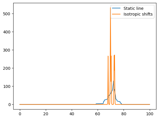
# Compute the spectrum for protons; only chemical shielding, including anisotropy effects
freqRange = 100
spec1H_aniso, freqs = nCalc.spectrum_1d('1H', effects=NMRFlags.STATIC, max_freq=freqRange, min_freq=0, bins=501)
# Now only the isotropic lines (as if spinning)
# We add a broadening to make the lines more visible
spec1H_iso, freqs = nCalc.spectrum_1d('1H', effects=NMRFlags.MAS, max_freq=freqRange, min_freq=0, bins=501,
                                      freq_broad=0.2)
fig = plt.figure()
ax = fig.add_subplot(111)

ax.plot(freqs, spec1H_aniso, label='Static line')
ax.plot(freqs, spec1H_iso, label='Isotropic shifts')

ax.legend()
<matplotlib.legend.Legend at 0x7f0d5c9956d0>
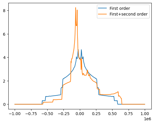
# Now let's look at the static quadrupolar line of 17O
freqRange = 1000000
spec17O_1, freqs = nCalc.spectrum_1d('17O', effects=NMRFlags.Q_1_ORIENT, max_freq=freqRange, min_freq=-freqRange, bins=501)
spec17O_s, freqs = nCalc.spectrum_1d('17O', effects=NMRFlags.Q_STATIC, max_freq=freqRange, min_freq=-freqRange, bins=501)
fig = plt.figure()
ax = fig.add_subplot(111)

ax.plot(freqs, spec17O_1, label='First order')
ax.plot(freqs, spec17O_s, label='First+second order')

ax.legend()
<matplotlib.legend.Legend at 0x7f0d5bfb8050>
# There's a number of other possible NMRFlags for various effects...
for fl in NMRFlags._fields:
    print(fl)
CS_ISO
CS_ORIENT
CS
Q_1_ORIENT
Q_2_SHIFT
Q_2_ORIENT_STATIC
Q_2_ORIENT_MAS
Q_2_STATIC
Q_2_MAS
Q_STATIC
Q_MAS
STATIC
MAS
7.1 - 2D spectra#
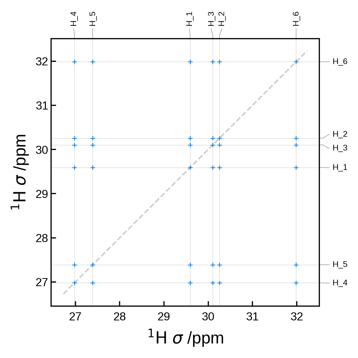
Minimal 2D NMR plot#
We can get a minimal 2D NMR plot simply by running:
from soprano.calculate.nmr.nmr import NMRData2D, NMRPlot2D, PlotSettings
atoms = ase_io.read('./tutorial_data/ethanol.magres')
nmr_data = NMRData2D(atoms, xelement = 'H')
plot = NMRPlot2D(nmr_data)
plot.plot();
Filtering the peaks by distance#
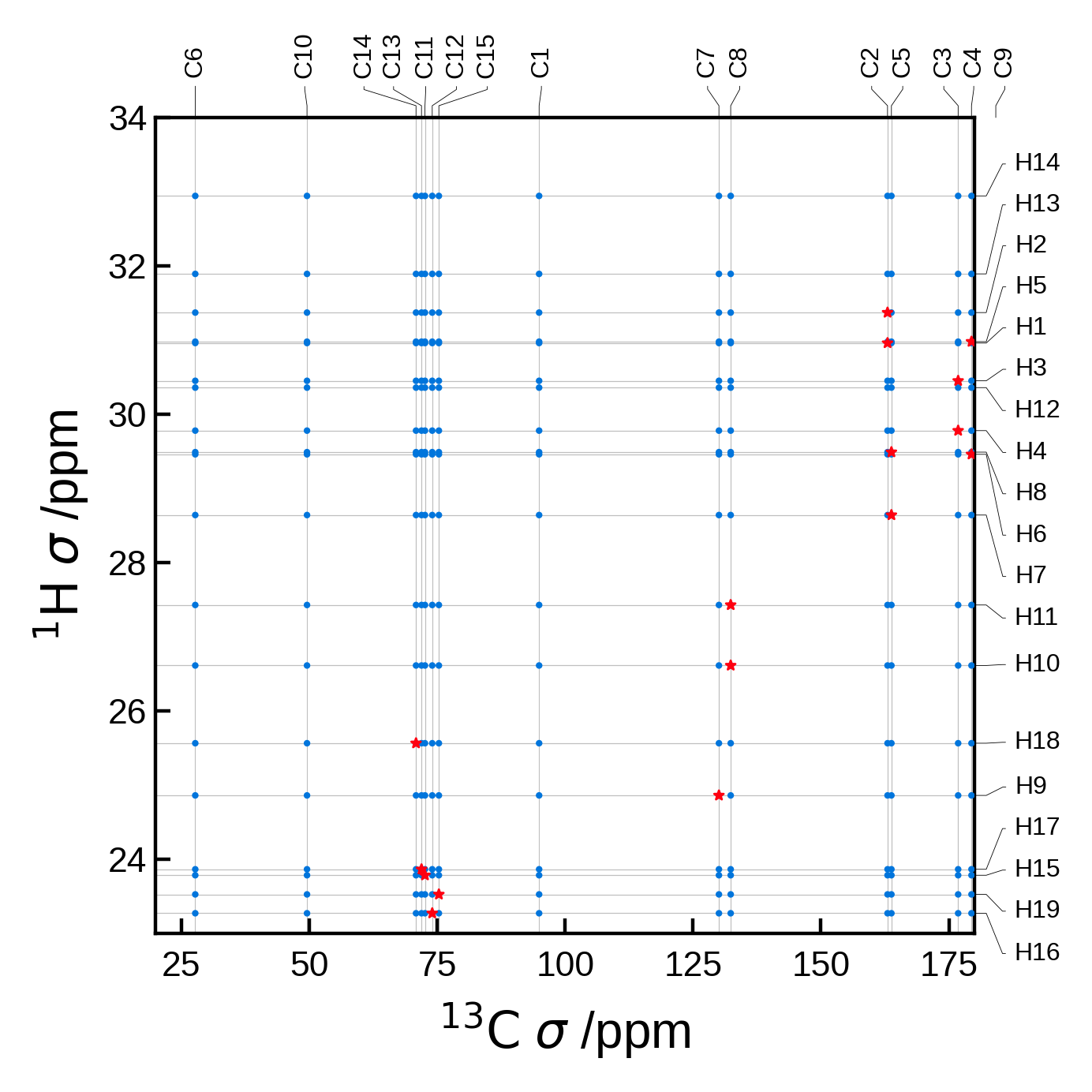
A common task is to filter the peaks by distance. This can be done by using the rcut argument in the NMRData2D object. This argument is a float that represents the maximum distance in Å to consider for the automatic peak finder.
For this example let’s use an atoms object with a lot more atoms, to see how the peak finder works with a more complex system.
We will plot all the C-H pairs in blue (circles) and those C-H pairs within 1.5 Å in red (stars).
edizum = ase_io.read('tutorial_data/EDIZUM.magres')
xlims = (20, 180)
ylims = (23, 34)

# To better see the difference, let's plot the data with and without a cut off radius.

# without any cut off radius:
nmr_data_all = NMRData2D(
    edizum,
    xelement = 'C',
    yelement = 'H',
    )
# There are 19 unique H and 15 unique C atoms in the unit cell = 285 pairs
# Note that there are actually 4 molecules in this unit cell, so we really have
# 4*19 * 4*15 = 4560 pairs, but these get identified as equivalent and then merged to 285.

print(f"The total number of C-H pairs is {len(nmr_data_all.peaks)}")
plot_settings = PlotSettings(
    marker_color='C0',
    marker = 'o',
    max_marker_size=1,
    xlim=xlims,
    ylim=ylims,
    )

plot = NMRPlot2D(nmr_data_all, plot_settings)
fig, ax = plot.plot()

# with a cut off radius:
rcut = 1.5 # Angstrom
nmr_data_cut = NMRData2D(
    edizum,
    xelement = 'C',
    yelement = 'H',
    rcut = rcut # ** here is where we set the cut off radius **
    )

print(f"The C-H pairs within rcut={rcut} Å is {len(nmr_data_cut.peaks)}")

# Now we can plot the data
plot_settings = PlotSettings(
    marker_color='C5',
    marker = '*',
    max_marker_size=5,
    show_labels=False, # no need to write them twice
    xlim=xlims,
    ylim=ylims,
    )
plot = NMRPlot2D(nmr_data_cut, plot_settings)
plot.plot(ax=ax);
The total number of C-H pairs is 285
The C-H pairs within rcut=1.5 Å is 19
More advanced 2D NMR plot#
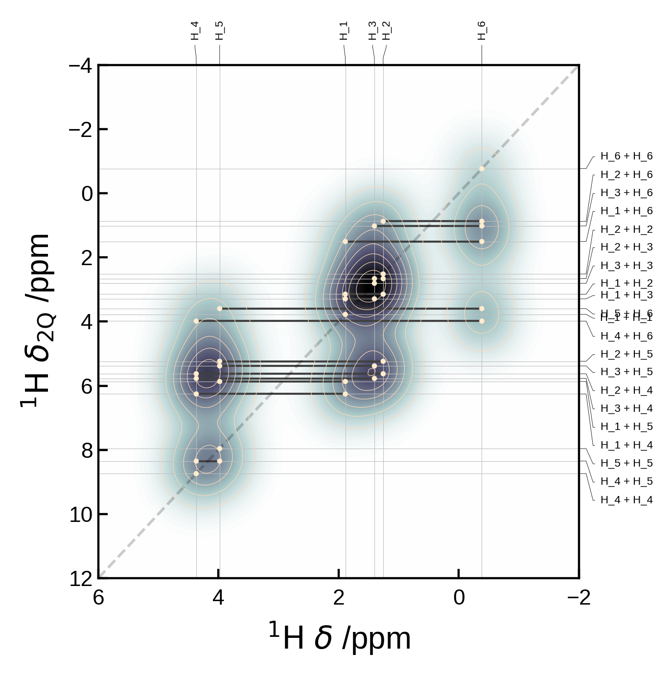
For a more complete example, let’s set a few more options explicitly. Below we plot an proton-proton double-quantum–single-quantum plot. Note that since we set the references explicitly, the plot will be converted from magnetic shielding \(\sigma\) to chemical shift \(\delta\).
# Extract the NMR data
nmr_data = NMRData2D(
            atoms,
            xelement = 'H',
            yelement = 'H', # if not specified, defaults to xelement
            isotopes= {'H': 1},
            references= {'H': 30.0}, # ppm
            gradients= {'H': -0.95}, # Nominally -1 given the formular to convert from shielding to shift
            yaxis_order= '2Q', # 1Q or 2Q for single- or double-quantum spectra
            )

# Set the plot settings
plot_settings = PlotSettings(
    xlim=(6, -2), # x-axis limits (note the reversed order here for shifts)
    ylim=(12, -4), # y-axis limits (note the reversed order here for shifts)
    marker='o', # marker style
    marker_color = 'blanchedalmond', # marker color
    max_marker_size=2, # maximum marker size (if fixed size, this will be the size)
    show_contour=True, # show contour lines
    contour_color='peachpuff', # contour line color
    contour_levels=10, # number of contour lines
    contour_linewidth=0.2, # contour line width
    show_heatmap=True, # show heatmap
    colormap='bone_r', # heatmap color scheme. Note that _r reverses the colormap. Other common colormaps are 'viridis', 'plasma', 'inferno', 'magma', 'cividis'
    heatmap_levels=100, # number of heatmap levels
    heatmap_grid_size=200, # heatmap grid size for broadening
    show_connectors=True, # show lines connecting two points at same y value
    label_fontsize=4, # label font size
    )
# Create the plot
plot = NMRPlot2D(nmr_data, plot_settings)
plot.plot();
WARNING: Elements {np.str_('C'), np.str_('O')} are not in the references dictionary and their reference will be set to zero. (/home/runner/work/soprano/soprano/soprano/properties/nmr/ms.py, line: 283)
Choosing which pairs to plot#
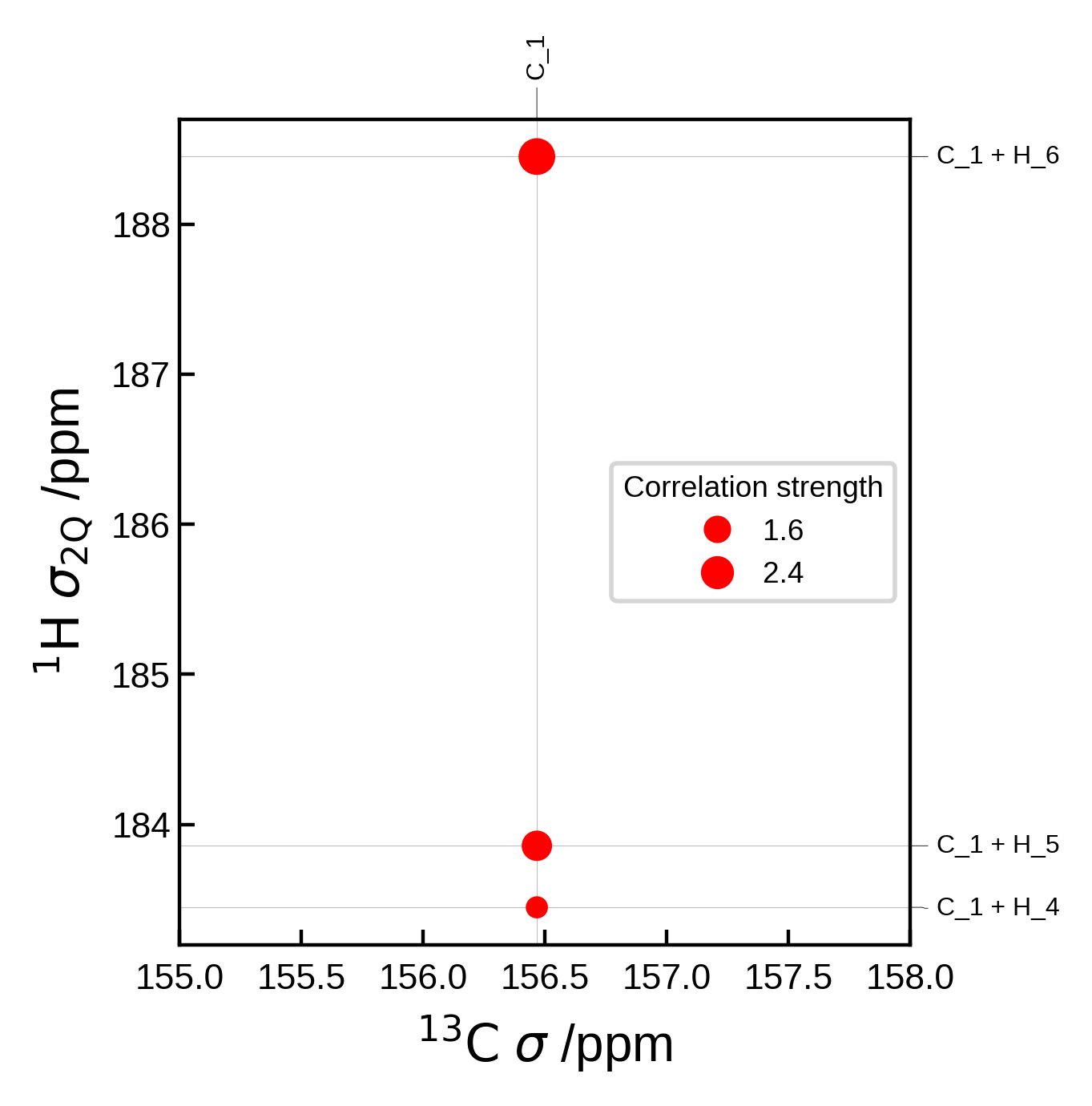
You might want to supply the pairs of sites together with a measure of their correlation strength. This can be done by supplying the pairs argument with a list of tuples of the form (i, j) and the markersizes argument. The markersizes argument should be a list of the same length as pairs and contain the size of the marker for each pair. The sizes are normalised to the maximum size in the list.
The pair indices must correspond to those of the atoms in the Atoms object.
# Here's an artificial example of how you might select custom pairs to plot
pairs = [(6,3), (6,4), (6,5)]
# and assign them different markersizes/correlation strengths to indicate the relative correlation strength
# (these are normalised internally such that the max absolute value is set to the max marker size)
markersizes=  [1,2,3]

xelement = 'C'
yelement = 'H'
yaxis_order = '2Q'
xlim = (155, 158)

plot_settings = PlotSettings(
    xlim=xlim,
    marker='o',
    marker_color = 'red',
    max_marker_size=60,
    show_legend=True,
)

# Extract and plot the data
nmr_data = NMRData2D(atoms, xelement = xelement, yelement = yelement, pairs=pairs, yaxis_order=yaxis_order, correlation_strengths=markersizes)
plot = NMRPlot2D(nmr_data, plot_settings)
plot.plot();
Custom peaks#
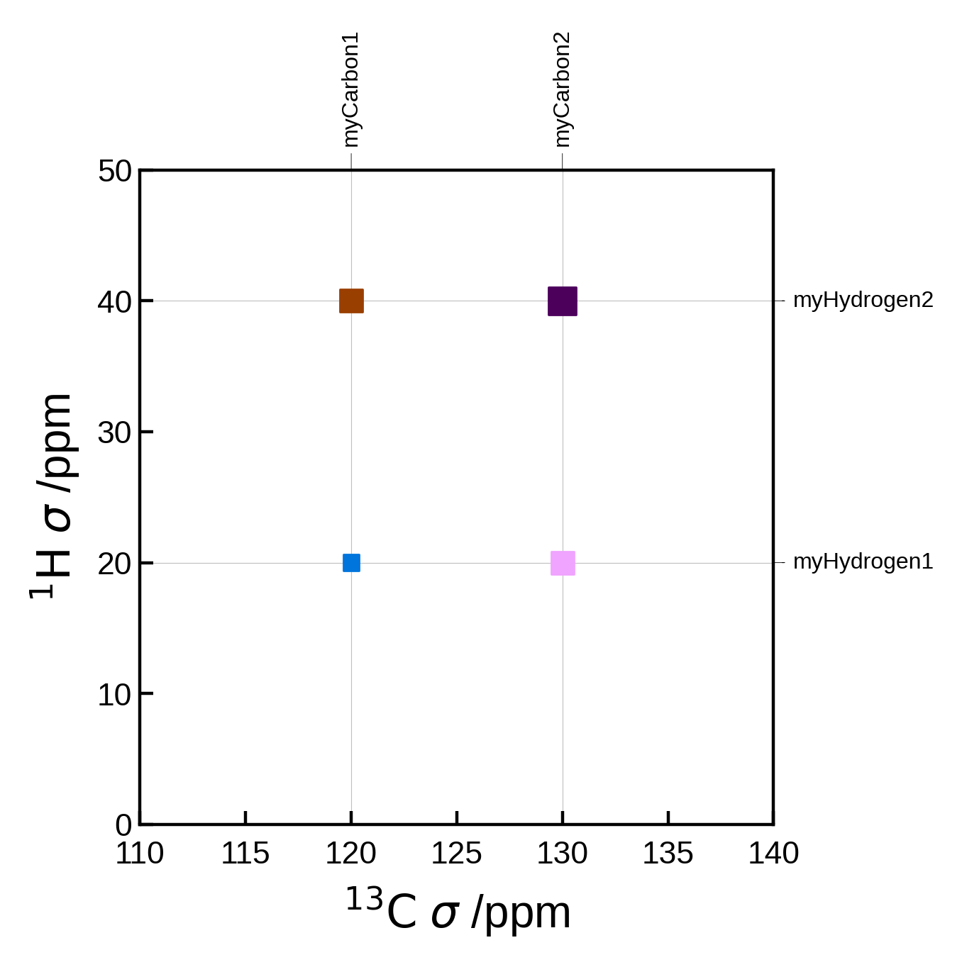
Instead of supplying pairs, we can instead supply the peaks as a list of Peak2D objects. This allows us to set the peak location, strength etc. directly. The pairs and markersizes arguments are ignored in this case.
One advantage of doing this is that you no longer need an Atoms object to plot the spectrum. This can be useful if you have a list of peaks from a different source.
from soprano.calculate.nmr.utils import Peak2D
# Artificial example of how you might define peaks if you have a list of carbon and hydrogen shieldings
C_ms = [120, 130]
H_ms = [20, 40]
peaks = []
for iC, C in enumerate(C_ms):
    for iH, H in enumerate(H_ms):
        peak = Peak2D(
                    C, # x position (ppm)
                    H, # y position (ppm)
                    f'myCarbon{iC+1}', # x label
                    f'myHydrogen{iH+1}', # y label
                    correlation_strength=iC + iH+1 # correlation strength (normalised). Here we just add the indices as an arbitrary example
                    )
        peaks.append(peak)

# we can also get creative and assign different colors to the peaks:
peaks[0].color = 'C0'
peaks[1].color = 'C1'
peaks[2].color = 'C2'
peaks[3].color = 'C3'

nmr_data = NMRData2D(
    None, # we don't need the atoms object here if we provide the peaks
    peaks=peaks,
    x_axis_label=r"$\mathrm{^{13}C}$ $\sigma$ /ppm", # We can use LaTeX here
    y_axis_label=r"$\mathrm{^{1}H}$ $\sigma$ /ppm",  # We can use LaTeX here
)

plot_settings = PlotSettings(
    marker='s', # square marker
    xlim=(110, 140),
    ylim=(0, 50),
    max_marker_size=50,
)
plot = NMRPlot2D(nmr_data, plot_settings)
plot.plot();
Editing peaks from automatic generation#
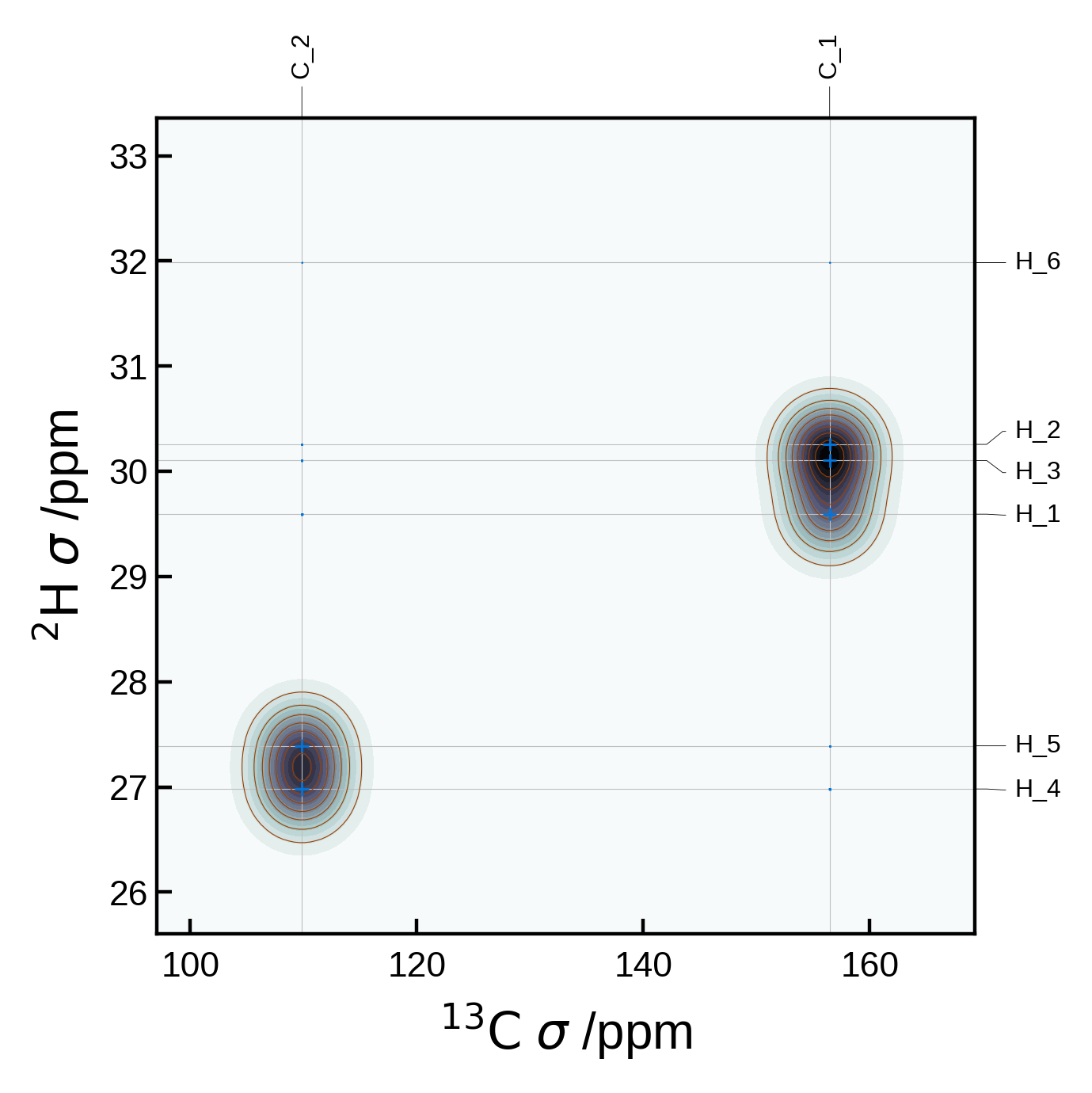
If you don’t want to create the Peak2D objects completely from scratch, we can get the automatically generated peaks, edit them and then plot them.
For example, here we use Soprano to compute the J-coupling values for each peak and use that to determine the correlation strength.
Though note that we could also have simply used correlation_strength_metric = jcoupling in the NMRData2D object to achieve the same result, for this simple case.
from soprano.properties.nmr.isc import JCIsotropy
isotopes = {'C': 13, 'H': 2}
# Extract the data (including the peaks)
nmr_data = NMRData2D(atoms, xelement = 'C', yelement = 'H', isotopes=isotopes)

# Now the peaks are available at `nmr_data.peaks`

# Loop over each peak and set the J-coupling for each peak to be the correlation strength
for peak in nmr_data.peaks:
    # Soprano wants the indices in ascending order
    i,j = sorted([peak.idx_x, peak.idx_y])
    # Get the J-coupling
    jcoup = JCIsotropy().get(atoms,tag = 'isc', sel_i = [i], sel_j = [j], isotopes = isotopes)
    # Set the correlation strength to the J-coupling
    peak.correlation_strength = jcoup[(i,j)]

# Plot settings
plot_settings = PlotSettings(
    show_heatmap=True,
    show_contour=True,
    )

plot = NMRPlot2D(nmr_data, plot_settings)
# plot
fig, ax = plot.plot()
Comparing in-built correlation strength metrics#
We can compare the different correlation strength metrics by plotting them all on the same plot. Below we plot the same 2D NMR plot as above, but with the correlation_strength_metric argument set to fixed, dipolar, jcoupling and inversedistance.
fig, axs = plt.subplots(2, 2, figsize=(10, 10))
axs = axs.flatten()
metrics = ['fixed', 'dipolar', 'jcoupling', 'inversedistance']

for i, metric in enumerate(metrics):
    nmr_data = NMRData2D(
        atoms,
        xelement = 'C',
        yelement = 'H',
        isotopes=isotopes,
        correlation_strength_metric=metric,
        references={'C': 175, 'H': 30, 'O': 0},
        )
    plot_settings = PlotSettings(
        show_markers=True,
        max_marker_size=80,
        marker_linewidth=1,
        show_heatmap=True,
        show_contour=True,
        x_broadening=5,
        y_broadening=0.2,
        colormap='bone_r' if metric != 'dipolar' else 'bone',
        contour_color='r',
        show_legend=True,
        )
    plot = NMRPlot2D(nmr_data, plot_settings)
    _ = plot.plot(ax=axs[i])
    # add title to each axis, adjusting the height to not overlap with the labels outside the axes
    axs[i].set_title(f'{metric.capitalize()} correlation strength', y=1.1)

plt.tight_layout()
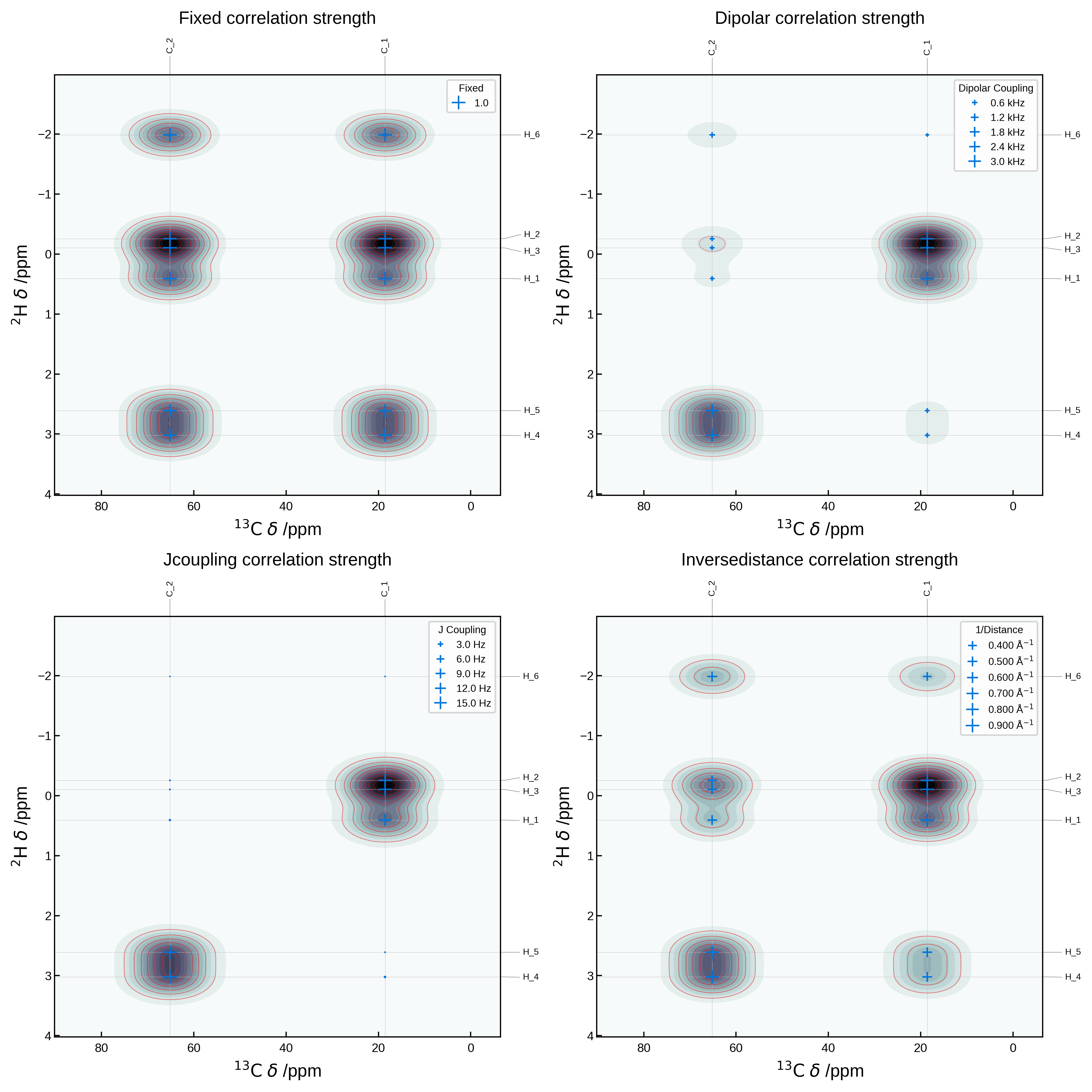
Combining 2D and 1D spectra#
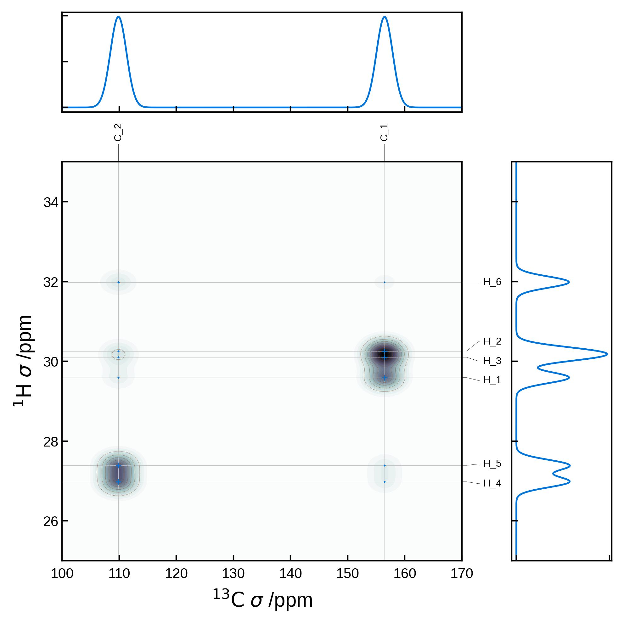
More complex plots are possible by first manually generating the matplotlib figure and axes and passing the axis to the NMRPlot2D class’ plot method. For example, we can create a customised plot in which we combine 2D and 1D spectra:
import matplotlib.pyplot as plt
from matplotlib.gridspec import GridSpec
from soprano.calculate.nmr.nmr import NMRCalculator, NMRFlags

# Common parameters
xlims = (100, 170)
ylims = (25, 35)
nbins = 501 # number of bins for the 1D plots and also the grid size for the 2D plot
x_broadening = 2.0
y_broadening = 0.2

# Compute the 1D spectrum for protons and carbons
nCalc = NMRCalculator(atoms) # We create the calculator here
# Set a powder averaging. Higher values of N mean finer average. Here we only care about the isotropic lines, so we can set N=1
nCalc.set_powder(N=1)
# proton spectrum
spec1H_iso, freqs1H   = nCalc.spectrum_1d('1H', effects=NMRFlags.MAS, max_freq=ylims[1], min_freq=ylims[0], bins=nbins, freq_broad=y_broadening)
# carbon spectrum
spec13C_iso, freqs13C = nCalc.spectrum_1d('13C', effects=NMRFlags.MAS, max_freq=xlims[1], min_freq=xlims[0], bins=nbins, freq_broad=x_broadening)

# Create a figure with the 2D plot and 2 1D plots above and to the right of the 2D plot
fig = plt.figure(figsize=(5,5))
# GridSpec is a more advanced way to create subplots with fine control over the layout
gs = GridSpec(2, 2, width_ratios=[4, 1], height_ratios=[1, 4])

# Create the 1D carbon plot at the top
ax1d_x = fig.add_subplot(gs[0, 0])
ax1d_x.plot(freqs13C, spec13C_iso, lw=1)
ax1d_x.set_xlim(xlims)
ax1d_x.set_xticklabels([])
ax1d_x.set_yticklabels([])

# Create the 1D proton plot on the right
ax1d_y = fig.add_subplot(gs[1, 1])
ax1d_y.plot(spec1H_iso, freqs1H, lw=1)
ax1d_y.set_ylim(ylims)
ax1d_y.set_xticklabels([])
ax1d_y.set_yticklabels([])

# Extract the 2D NMR data
nmr_data_2d = NMRData2D(
    atoms,
    xelement='C',
    yelement='H',
    correlation_strength_metric='dipolar')

# Create the 2D plot axis
ax2d = fig.add_subplot(gs[1, 0])

# Set the plot settings
plot_settings = PlotSettings(
    xlim=xlims,
    ylim=ylims,
    show_heatmap=True,
    show_contour=True,
    x_broadening=x_broadening, # can use the same broadening settings
    y_broadening=y_broadening, # can use the same broadening settings
    heatmap_levels=40,
    heatmap_grid_size = nbins,
    colormap='bone',
    contour_levels=10,
    contour_linewidth=0.1,
    )
# Plot the 2D data on the 2D axis
plot = NMRPlot2D(nmr_data_2d, plot_settings)
plot.plot(ax = ax2d)

#increase space between subplots
plt.subplots_adjust(wspace=0.2, hspace=0.2)
8 - Euler angles#
Euler angles are commonly used to describe the orientation of an NMR tensor in space. Three angles, \(\alpha\), \(\beta\) and \(\gamma\), are defined as the rotations around successive axes, depending on the convention used. The most common convention in NMR is the ZYZ convention, where the rotations are performed around the \(z\) axis, then the \(y\) axis and finally the \(z\) axis again.
Euler angles can be a major source of confusion when comparing different software packages, as the conventions can vary and the handling of ambiguous cases differs greatly. In Soprano we follow the excellent work of Svenningsson & Mueller (2023) in their TensorView for MATLAB package. They provide a comprehensive explanation of how to deal with edge-cases and equivalencies in relative Euler angles between NMR tensors.
Some of the choices to be aware of are:
The order of the rotations (ZYZ or ZXZ are supported).
Active or passive: this is a choice of whether the tensor itself is rotated (active) or the reference frame is rotated (passive).
The ordering of the tensor eigenvalues: the standard convention for EFG tensors is the “NQR” ordering, i.e. \(|V_3| \geq |V_2| \geq |V_1|\), where these are the principal components of the EFG tensor. There are several conventions for ordering magnetic shielding tensor principal components. A commonly used one is “Haeberlen” ordering in which \(|\delta_{zz} - \delta_{\mathrm{iso}}| \geq |\delta_{xx} - \delta_{\mathrm{iso}}| \geq |\delta_{yy} - \delta_{\mathrm{iso}}|\), where \(\delta_{zz}\) etc. are the principal components of the chemical shift tensor and \(\delta_{\mathrm{iso}}\) is the isotropic component. Common conventions are nicely explained here.
As explained in the TensorView for MATLAB paper, even with these choices set, there are still ambiguities in the Euler angles. In the general case, there are four equivalent sets of Euler angles for a given tensor. For relative Euler angles, there are 16 equivalent sets!
Soprano provides utilities to compute Euler angles, specifying your choice of rotation order, active vs passive and the tensor ordering. Soprano also allows you to calculate equivalent Euler angles to make cross-software comparisons easier.
General NMR tensor#
Soprano provides a general NMRTensor class that can be used in isolation, but also some convenience methods for dealing with NMR tensors from e.g. a .magres file. First let’s look at the general case:
from soprano.nmr import NMRTensor

# Let's create a tensor such as (this is actually a chemical shielding tensor from the ethanol.magres file
# but it can be any 3x3 tensor)

data = np.array([
    [30.29817962,  1.20510693,  3.67274493],
    [ 1.96313295, 27.57652505,  2.57545224],
    [ 4.21834132,  2.16271308, 30.90315252]])

t = NMRTensor(data)
# Now t is an NMRTensor object. We can extract a variety of properties of this tensor
# and perform updates to e.g. the tensor ordering


# These are the ordering conventions available in Soprano:
orders = {'i': 'Increasing', 'd': 'Decreasing', 'n': 'NQR', 'h': 'Haeberlen'}
# We can loop over the orderings
for o, oname in orders.items():
    # Update tensor's order
    t.order = o
    # and print the Euler angles for each combination of {ZYZ,ZXZ} and {active, passive}
    print("{0} order".format(oname))
    print("Eigenvalues: {0:.2f}, {1:.2f}, {2:.2f}".format(*t.eigenvalues))
    print("ZYZ (active)  α={0:6.1f}, β={1:6.1f}, γ={2:6.1f} (deg)".format(*t.euler_angles(convention='zyz', passive=False)*180/np.pi))
    print("ZYZ (passive) α={0:6.1f}, β={1:6.1f}, γ={2:6.1f} (deg)".format(*t.euler_angles(convention='zyz', passive=True)*180/np.pi))
    print("ZXZ (active)  α={0:6.1f}, β={1:6.1f}, γ={2:6.1f} (deg)".format(*t.euler_angles(convention='zxz', passive=False)*180/np.pi))
    print("ZXZ (passive) α={0:6.1f}, β={1:6.1f}, γ={2:6.1f} (deg)".format(*t.euler_angles(convention='zxz', passive=True)*180/np.pi))
    print()
Increasing order
Eigenvalues: 26.19, 27.04, 35.55
ZYZ (active)  α=  28.0, β=  45.3, γ=  26.8 (deg)
ZYZ (passive) α= 153.2, β=  45.3, γ= 152.0 (deg)
ZXZ (active)  α= 118.0, β=  45.3, γ= 116.8 (deg)
ZXZ (passive) α=  63.2, β=  45.3, γ=  62.0 (deg)

Decreasing order
Eigenvalues: 35.55, 27.04, 26.19
ZYZ (active)  α= 243.7, β=  50.6, γ= 155.4 (deg)
ZYZ (passive) α=  24.6, β=  50.6, γ= 296.3 (deg)
ZXZ (active)  α= 333.7, β=  50.6, γ=  65.4 (deg)
ZXZ (passive) α= 114.6, β=  50.6, γ= 206.3 (deg)

NQR order
Eigenvalues: 26.19, 27.04, 35.55
ZYZ (active)  α=  28.0, β=  45.3, γ=  26.8 (deg)
ZYZ (passive) α= 153.2, β=  45.3, γ= 152.0 (deg)
ZXZ (active)  α= 118.0, β=  45.3, γ= 116.8 (deg)
ZXZ (passive) α=  63.2, β=  45.3, γ=  62.0 (deg)

Haeberlen order
Eigenvalues: 26.19, 27.04, 35.55
ZYZ (active)  α=  28.0, β=  45.3, γ=  26.8 (deg)
ZYZ (passive) α= 153.2, β=  45.3, γ= 152.0 (deg)
ZXZ (active)  α= 118.0, β=  45.3, γ= 116.8 (deg)
ZXZ (passive) α=  63.2, β=  45.3, γ=  62.0 (deg)
  WARNING:  Isotropic value(s) are not zero but NQR order is requested.
If you're dealing with an EFG tensor, then check it carefully since these should be traceless.
Sorting by absolute values.
 (/home/runner/work/soprano/soprano/soprano/nmr/utils.py, line: 64)
We have seen how to specify your choice of conventions in Soprano to calculate Euler angles. However, as discussed earlier, there are four equivalent Euler angle sets for any choice of {ZYZ,ZXZ}, {active, passive}, and ordering convention. Understanding this can be very important when comparing results from different codes.
You can access equivalent Euler angles in Soprano like this:
# For example, for the ZYZ, active, Haeberlen convention tensor:
t.order = 'h'
equivalent_eulers = t.equivalent_euler_angles('zyz', passive=False) * 180 / np.pi

# We can print these out neatly:
for eulers in equivalent_eulers:
    print('α={0:6.1f}, β={1:6.1f}, γ={2:6.1f} (deg)'.format(*eulers))
α=  28.0, β=  45.3, γ=  26.8 (deg)
α=  28.0, β=  45.3, γ= 206.8 (deg)
α= 208.0, β= 134.7, γ= 153.2 (deg)
α= 208.0, β= 134.7, γ= 333.2 (deg)
NMR tensors from .magres data#
We saw earlier in this tutorial how magnetic shielding, EFG, dipolar coupling and J-coupling tensors could be extracted from a .magres file and analysed using Soprano. Here we explain how to access the Euler angles from these tensors and how different default orderings apply.
Chemical shielding tensors#
If you simply want the Euler angles according to the default ordering convention in Soprano for MS tensors (Haeberlen), for all sites in your magres file you can simply do:
from soprano.properties.nmr import MSEuler

all_eulers = MSEuler.get(C2H6O, order='h', convention='zyz', passive=False)

# NB that since these are the default settings for the MS tensors,
# you can achieve the same using simply:
all_eulers=  MSEuler.get(C2H6O)

print(all_eulers * 180 / np.pi)
[[ 27.96235601  45.33901509  26.83660999]
 [272.66415652  77.36879495  93.22520173]
 [182.04368043  35.14497966 166.45558554]
 [182.66142427  83.1949885  115.14989736]
 [191.97626819  50.93125971 125.47393484]
 [299.07186816  42.28810672  25.35033859]
 [ 93.10412193  47.43018725 152.96615397]
 [  9.25627104  54.93258925  41.36551806]
 [183.04713505  59.54692522 125.9519578 ]]
However, if you want to compute relative Euler angles, then you can instead first extract the NMRTensor objects and work directly with them. For example:
# get a list of NMRTensor objects with Haeberlen ordering:
ms_tensors = MSTensor().get(C2H6O)

print(f"There are {len(ms_tensors)} tensors in the ms_tensors list")

# To get the Euler angles (in degrees) for e.g first atom, as before you can do:
eulers_0 = ms_tensors[0].euler_angles('zyz', passive=False) * 180 / np.pi
print(eulers_0)

# or the relative Euler angles between the first two atoms:
eulers_0_to_1 = ms_tensors[0].euler_to(ms_tensors[1]) * 180 / np.pi
print(eulers_0_to_1)
There are 9 tensors in the ms_tensors list
[27.96235601 45.33901509 26.83660999]
[226.25350967  81.78516894  36.20814598]
Equivalent Euler angles#
As discussed earlier, in the general case, the Euler angles that describe the rotation from one NMR tensor to another are not unique. In fact, for a given choice of conventions, there can be up to 16 equivalent Euler angle sets all correctly describing the same rotation.
For example, the rotation between the MS shielding tensor of atom 0 to that of atom 1 can be described by any of:
equivalent_eulers_0_to_1 = ms_tensors[0].equivalent_euler_to(ms_tensors[1])

# This is just to print them out neatly, in degrees:
print("α\t\tβ\t\tγ (deg)")
for eulers in equivalent_eulers_0_to_1:
    print('{0:6.2f}\t\t {1:6.2f}\t\t {2:6.2f}'.format(*eulers* 180 / np.pi))
α		β		γ (deg)
226.25		  81.79		  36.21
 46.25		  98.21		 323.79
 46.25		  98.21		 143.79
226.25		  81.79		 216.21
133.75		  98.21		 216.21
313.75		  81.79		 143.79
313.75		  81.79		 323.79
133.75		  98.21		  36.21
313.75		  98.21		 216.21
133.75		  81.79		 143.79
133.75		  81.79		 323.79
313.75		  98.21		  36.21
 46.25		  81.79		  36.21
226.25		  98.21		 323.79
226.25		  98.21		 143.79
 46.25		  81.79		 216.21
EFG tensors#
The approach to accessing EFG tensor Euler angles is exactly the same, though it’s important to note that the default ordering for EFG tensors follows the NQR convention (\(|V_{xx}| \geq |V_{yy}| \geq |V_{zz}|\))!
If you’re using Simpson, then the ordering is \(|V_{yy}| \geq |V_{xx}| \geq |V_{zz}|\) - i.e. the xx and yy components are swapped compared to the NQR convention. Since the EFG tensor is traceless (-> isotropy = 0), we can use the “Haeberlen” ordering in order to reproduce the Simpson convention.
from soprano.properties.nmr import EFGEuler

all_eulers = EFGEuler.get(C2H6O, order='n', convention='zyz', passive=False)

# NB that since these are the default settings for the EFG tensors,
# you can achieve the same using simply:
all_eulers=  EFGEuler.get(C2H6O)

print(all_eulers * 180 / np.pi)
[[ 11.03244319  53.8688531  124.66006684]
 [281.370063    58.60389462 177.2437768 ]
 [193.17945823  54.80749091  63.11651013]
 [192.58906551  54.86121432   1.71828894]
 [282.0979964   58.46767793 125.27455202]
 [283.02612009  54.60580544 119.15653422]
 [107.1814723   53.91168656  32.42758192]
 [ 13.77889019  54.51695231 129.73651409]
 [146.57430779  44.36396799  94.77789967]]
To follow the Simpson convention you can add or subtract 90 degrees from either the \(\alpha\) or \(\gamma\) Euler angle, depending on the situation - see note here. Alternatively, use the Haeberlen ordering in Soprano since that gives the same result as the Simpson convention for EFG tensors.
all_eulers = EFGEuler.get(C2H6O, order='h', convention='zyz', passive=False)
print(all_eulers * 180 / np.pi)
[[ 11.03244319  53.8688531   34.66006684]
 [281.370063    58.60389462  87.2437768 ]
 [193.17945823  54.80749091 153.11651013]
 [192.58906551  54.86121432  91.71828894]
 [282.0979964   58.46767793  35.27455202]
 [283.02612009  54.60580544  29.15653422]
 [107.1814723   53.91168656 122.42758192]
 [ 13.77889019  54.51695231  39.73651409]
 [146.57430779  44.36396799   4.77789967]]
Relative Euler angles between MS and EFG tensors#
This follows the same pattern as before: first extracting the NMRTensor objects and then using the euler_to methods to calculate the relative Euler angles between them.
For example, looking each atom, we can compute the rotation to get from its MS tensor to its EFG tensor like this:
ms_tensors = MSTensor.get(C2H6O)
efg_tensors = EFGTensor.get(C2H6O)

print('Euler angles from the MS to EFG tensors for each atom:')
print("α\t\tβ\t\tγ (deg)")
for ms, efg in zip(ms_tensors, efg_tensors):
    eulers = ms.euler_to(efg)
    print('{0:6.2f}\t\t {1:6.2f}\t\t {2:6.2f}'.format(*eulers* 180 / np.pi))
Euler angles from the MS to EFG tensors for each atom:
α		β		γ (deg)
  4.13		  15.41		  89.09
 22.31		  20.41		  65.02
 45.14		  21.12		  39.52
201.89		  29.77		  48.35
318.10		  21.50		 153.58
158.30		  17.14		 104.76
 22.47		  12.65		  89.11
145.38		   3.72		 123.64
236.61		  81.84		 148.84
Dipolar Coupling#
from soprano.properties.nmr import DipolarTensor, DipolarEuler
# Let's say we only want the dipolar couplings between the 1st and 5th atoms:
ij = (1,5)

dip_eulers = DipolarEuler().get(C2H6O, degrees=True)[ij]
print(f"Euler angles for dipolar coupling between atoms\n{C2H6O[ij[0]]} and \n{C2H6O[ij[1]]}:\n {dip_eulers}")

# Now let's get the dipolar tensor for the same pair of atoms
dip_tensor = DipolarTensor().get(C2H6O)[ij]
print()
print(f"Dipolar tensor for dipolar coupling between atoms\n{C2H6O[ij[0]]} and \n{C2H6O[ij[1]]}:\n {dip_tensor.data}")
Euler angles for dipolar coupling between atoms
Atom('H', [np.float64(0.182454), np.float64(-0.924201), np.float64(0.559623)], index=1) and
Atom('H', [np.float64(1.060671), np.float64(0.677653), np.float64(2.297066)], index=5):
 [61.26622906 46.43614059  0.        ]

Dipolar tensor for dipolar coupling between atoms
Atom('H', [np.float64(0.182454), np.float64(-0.924201), np.float64(0.559623)], index=1) and
Atom('H', [np.float64(1.060671), np.float64(0.677653), np.float64(2.297066)], index=5):
 [[ 4767.38285255 -4977.57111273 -5398.8978314 ]
 [-4977.57111273 -1582.67354136 -9847.50475887]
 [-5398.8978314  -9847.50475887 -3184.70931119]]

